In short, data is any information that can be stored and analyzed to extract meaning or insights.
It is difficult to define such a broad concept, but the definition that I like it that data is a collection (or any set) of information, such as characters, numbers, symbols, words, files (text files, images, audio files), etc, that represent measurements, observations, or descriptions, that are gathered and stored for some purpose. https://www.mathsisfun.com/data/data.htmlhttps://www.computerhope.com/jargon/d/data.htm
It's data that doesn't fit easily into a spreadsheet or a relational database.
The line between Semi-structured data and Unstructured data has always been unclear. Semi-structured data is usually referred to as information that is not structured in a traditional database but contains some organizational properties that make its processing easier.
Examples of structured data include:
Quantative data:
Weather forecast data: Measurements of temperature, precipitation (in millimeters (mm)), atmospheric pressure, wind speed, cloud coverage
Seismic data: Measurement of ground movement caused by seismic activity.
Housing data: Gattered housing data composed, for example, by Price, Area of the house, Number of rooms, House age, Area population, Avg. Income of residents of the city
Numeric financial information and Market reports
Another good example of structured data is a company's database where the company stores all the data that is usually associated with the ERP (Enterprise resource planning: A suite of integrated applications that an organization can use to collect, store, manage, and interpret data from many business activities), such as:
Human resource data: For example, an «Employees» table: id, fname, lname, dob, email, phone_number, address
Customer data (Customer relationship management (CRM)): «Client» table
Text files: Word docs, PowerPoint presentations, Email, Chat logs, Text messages, Customer reviews, News articles, etc.
Email: There’s some internal metadata structure, so it’s sometimes called semi-structured, but the message field is unstructured and difficult to analyze with traditional tools.
Media files(Images, Audio, and Video files): Satellite images, surveillance images/videos, Call recordings (Call logs), Music audios/videos, Locations, etc.
Some sources of data are:
Social Media data: Data from social networking sites like Facebook, Twitter, and LinkedIn
Mobile data: Text messages
Call centers data
For example, NoSQL documents are considered to be semi-structured data since they contain keywords that can be used to process the documents easier. https://www.youtube.com/watch?v=dK4aGzeBPkk
It is important to highlight that the huge increase in data in the last 10 years has been driven by the increase in unstructured data. Currently, some estimations indicate that there are around 300 exabytes of data, of which around 80% is unstructured data.
The prefix exa indicates multiplication by the sixth power of 1000 ().
Some sources also suggest that the amount of data is doubling every 2 years.
There are four Levels of Measurement in research and statistics: Nominal, Ordinal, Interval, and Ratio.
In Practice:
Most schemes accommodate just two levels of measurement: nominal and ordinal
There is one special case: dichotomy (otherwise known as a "boolean" attribute)
Values have meaningful order
Distance between values is defined
Mathematical operations make sense
(Values can be used to perform mathematical operations)
There is a meaning ful zero-point
Values can be used to perform statistical computations
Example
Comparison operators
Addition and subtrac tion
Multiplica tion and division
"Counts", aka, "Fre quency of Distribu tion"
Mode
Median
Mean
Std
Nominal
Values serve only as labels. Also called "categorical", "enumerated", or "discrete". However, "enumerated" and "discrete" imply order
✘
✘
✘
✘
✘
✘
✔
✔
✘
✘
✘
Values don't have any meaningful order
No distance between values is defined
Values don't carry any mathematical meaning
Values cannot be used to perform many statistical computations, such as mean and standard deviation
Even if the values are numbers. For example, if we want to categorize males and females, we could use a number of 1 for male, and 2 for female. However, the values of 1 and 2 in this case don't have any meaningful order or carry any mathematical meaning. They are simply used as labels. https://www.statisticssolutions.com/data-levels-and-measurement/
For an «outlook» attribute from weather data, potential values could be "sunny", "overcast", and "rainy".
Ordinal
Ordinal attributes are called "numeric", or "continuous", however "continuous" implies mathematical continuity
✔
✘
✔
✘
✘
✘
✔
✔
✔
✘
✘
Values have a meaningful order
No distance between values is defined
Only comparison operators make sense
Mathematical operations such as addition, subtraction, multiplication, etc. do not make sense
For example, an «Education level» attribute with possible values of «high school», «undergraduate degree», and «graduate degree». There is a definitive order to the categories (i.eº., graduate is higher than undergraduate, and undergraduate is higher than high school), but we cannot make any other arithmetic assumption. For instance, we cannot assume that the difference in education level between undergraduate and high school is the same as the difference between graduate and undergraduate.
Distinction between nominal and ordinal not always clear (e.g., attribute "outlook")
A «temperature» attribute in weather data with potential values fo: "hot" > "warm" > "cool"
Interval
✔
✔
✔
✔
✘
✘
✔
✔
✔
✔
✔
Distance between values is defined. In other words, we can quantify the difference between values
Comparison operators make sense
Addition, subtraction, make sense
Multiplication, and division do not make sense
Interval variables often do not have a meaningful zero-point.
(not sure)
An example of an interval variable would be a «Temperature» attribute. We can correctly assume that the difference between 70 and 80 degrees is the same as the difference between 80 and 90 degrees. However, the mathematical operations of multiplication and division do not apply to interval variables. For instance, we cannot accurately say that 100 degrees is twice as hot as 50 degrees. Additionally, interval variables often do not have a meaningful zero-point. For example, a temperature of zero degrees (on Celsius and Fahrenheit scales) does not mean a complete absence of heat.
An interval variable can be used to compute commonly used statistical measures such as the average (mean), standard deviation, and the Pearson correlation coefficient. https://www.statisticssolutions.com/data-levels-and-measurement/
a «Temperature» attribute composed by numeric measures of such property
Ratio
✔
✔
✔
✔
✔
✔
✔
✔
✔
✔
✔
All arithmetic operations are possible on a ratio variable
Ratio variables have a meaningful zero-point
An example of a ratio variable would be weight (e.g., in pounds). We can accurately say that 20 pounds is twice as heavy as 10 pounds. Additionally, ratio variables have a meaningful zero-point (e.g., exactly 0 pounds means the object has no weight).
A ratio variable can be used as a dependent variable for most parametric statistical tests such as t-tests, F-tests, correlation, and regression. https://www.statisticssolutions.com/data-levels-and-measurement/
The «weight» (e.g., in pounds)
Other examples: gross sales and income of a company.
An example, also known in statistics as an observation, is an instance of the phenomenon that we are studying. An observation is characterized by one or a set of attributes (variables).
In data science, we record observations on the rows of a table.
For example, imaging that we are recording the vital signs of a patient. For each observation we would record the «date of the observation», the «patient's heart» rate, and the «temperature»
What is a dataset
[Noel Cosgrave slides]
A dataset is typically a matrix of observations (in rows) and their attributes (in columns).
It is usually stored as:
Flat-file (comma-separated values (CSV)) (tab-separated values (TSV)). A flat file can be a plain text file or a binary file.
Spreadsheets
Database table
It is by far the most common form of data used in practical data mining and predictive analytics. However, it is a restrictive form of input as it is impossible to represent relationships between observations.
What is Metadata
Metadata is information about the background of the data. It can be thought of as "data about the data" and contains: [Noel Cosgrave slides]
Description of the variables.
Information about the data types for each variable in the data.
Restrictions on values the variables can hold.
What is Data Science
There are many different terms that are related. It is actually hard to define and differentiate some of these related disciplines such as:
Artificial intelligence (AI)
Data Science - Data Analysis - Data Analytics - Predictive Data Analytics - Data Mining - Machine Learning - Big Data - Business Analytics.
Artificial intelligence (AI) is a broader field that encompasses various subfields, including machine learning, natural language processing, computer vision, robotics, and more. [ChatGPT]
At a high level, the goal of AI is to create intelligent machines that can perform tasks that typically require human-level intelligence, such as perception, reasoning, decision-making, and natural language understanding. [ChatGPT]
Data Science
Data Sciences is a very broad discipline (an umbrella term) that involves (encompasses) many subsets such as Data Analysis, Data Analytics, Data Mining, Machine Learning, Big data (could also be included), and several other related disciplines.
Data analysis is still a very broad process that includes many multi-disciplinary stages, it goes from: (that are not usually related to Data Analytics or Data Mining)
Data Transformation: The data is transformed or consolidated into forms that are appropriate or valid for mining by performing various aggregation operations. http://troindia.in/journal/ijcesr/vol3iss3/36-40.pdf
We can say that Data Mining is a Data Analysis subset. It's the process of (1) Discovering hidden patterns in data and (2) Developing predictive models, by using statistics, learning algorithms, and data visualization techniques.
Common methods in data mining are: See Styles of Learning - Types of Machine Learning section
Big Data
Big data describes a massive amount of data that has the potential to be mined for information but is too large to be processed and analyzed using traditional data tools.
Machine Learning
Machine learning is one of the most important subfields of AI, as it provides a way for computers to automatically learn and improve from experience or data, rather than having to be re-programmed to do so. [ChatGPT]
Una de las definiciones más citadas es la definición de Tom Mitchell. This author provides in his book Machine Learning a definition in the opening line of the preface:
Tom Mitchell
The field of machine learning is concerned with the question of how to construct computer programs that automatically improve with experience.
So, in short we can say that ML is about writingcomputer programs that improve themselves.
Tom Mitchell also provides a more complex and formal definition:
Tom Mitchell
A computer program is said to learn from experience E with respect to some class of tasks T and performance measure P, if its performance at tasks in T, as measured by P, improves with experience E.
Don't let the definition of terms scare you off, this is a very useful formalism. It could be used as a design tool to help us think clearly about:
P: The number (or fraction) of emails correctly classified as spam/not spam.
Machine Learning and Data Mining are terms that overlap each other. This is logical because both use the same techniques (weel, many of the techniques uses in Data Mining are also use in ML). I'm talking about Supervised and Unsupervised Learning algorithms (that are also called Supervised ML and Unsupervised ML algorithms).
The difference is that in ML we want to construct computer programs that automatically improve with experience (computer programs that improve themselves)
We can, for instance, use a Supervised learning algorithm (Naive Bayes, for example) to build a model that, for example, classifies emails as spam or no-spam. So we can use labeled training data to build the classifier and then use it to classify unlabeled data.
So far, even if this classifier is usually called an ML classifier, it is NOT strictly a ML program. It is just a Data Mining or Predictive data analytics task. It's not a strict ML program because the classifier is not automatically improving itself with experience.
Now, if we are able to use this classifier to develop a program that automatically gathers and adds more training data to rebuild the classifier and updates the classifier when its performance improves, this would now be a strict ML program; because the program is automatically gathering new training data and updating the model so it will automatically improve its performance.
Supervised learning is the process of using training data (training data/labeled data: input (x) - output (y) pairs) to produce a mapping function () that allows mapping from the input variable () to the output variable (). The training data is composed of input (x) - output (y) pairs.
Put more simply, in Supervised learning we have input variables () and an output variable () and we use an algorithm that is able to produce an inferred mapping function from the input to the output.
The goal is to approximate the mapping function so well that when we have new input data (), we can predict the output variable .
The dependent variable is the variable that is to be predicted (). An independent variable is the variable or variables that is used to predict or explain the dependent variable ().
It is not so easy to see and understand the mathematical conceptual difference between Regression and Classification techniques. In both methods, we determine a function from an input variable to an output variable. It is clear that regressions methods predict continuous variables (the output variable is continuous), and classification predicts discrete variables. Now, if we think about the mathematical conceptual difference, we must notice that regression is estimating the mathematical function that most closely fits the data. In some classification methods, it is clear that we are not estimating a mathematical function that fits the data, but just a method/algorithm/mapping_function (no sé cual sería el término más adecuado) that allows us to map the input to the output. This is, for example, clear in K-Nearest Neighbors where the algorithm doesn't generate a mathematical function that fits the data but only a mapping function (de nuevo, no sé si éste sea el mejor término) that actually (in the case of KNN) relies on the data (KNN determines the class of a given unlabeled observation by identifying the k-nearest labeled observations to it). So, the mapping function obtained in KNN is attached to the training data. In this case, is clear that KNN is not returning a mathematical function that fits the data. In Naïve Bayes, the mapping function obtained is not attached to the data. That is to say, when we use the mapping function generate by NB, this doesn't require the training data (of course we require the training data to build the NB Mapping function, but not to apply the generated function to classify a new unlabeled observation which is the case of KNN). However, we can see that the mathematical concept behind NB is not about finding a mathematical function that fits the data but it relies on a probabilistic approach (tengo que analizar mejor lo último que he dicho aquí sobre NB). Now, when it comes to an algorithm like Decision Trees, it is not so clear to see and understand the mathematical conceptual difference between Regression and Classification. in DT, I think that (even if the output is a discrete variable) we are generating a mathematical function that fits the data. I can see that the method of doing so is not so clear as in the case of, for example, Linear regression, but it would in the end be a mathematical function that fits the data. I think this is why, by doing simples variation in the algorithms, decision trees can also be used as a regression method.
De hecho, Regression and classification methods are so closely related that:
A classification algorithm may predict a continuous value, but the continuous value is in the form of a probability for a class label.
Logistic Regression: Contrary to popular belief, logistic regression IS a regression model. The model builds a regression model to predict the probability that a given data entry belongs to the category numbered as "1". Just like Linear regression assumes that the data follows a linear function, Logistic regression models the data using the sigmoid function. https://www.geeksforgeeks.org/understanding-logistic-regression/
There are methods for implementing Regression using classification algorithms:
For example, the price of a house may be predicted using regression techniques.
Quizá podríamos decir que Regression analysis is the process of finding the mathematical function that most closely fits the data. The most common form of regression analysis is linear regression, which is the process of finding the line that most closely fits the data.
The purpose of regression analysis is to: [Noel]
Predict the value of the dependent variable as a function of the value(s) of at least one independent variable.
Explain how changes in an independent variable are manifested in the dependent variable
Linear Regression
Decision Tree Regression
Support Vector Machines (SVM): It can be used for classification and regression analysis
Neural Network Regression
Regression algorithms are used for:
Prediction of continuous variables: future prices/cost, incomes, etc.
Housing Price Prediction: For example, a regression model could be used to predict the value of a house based on location, number of rooms, lot size, and other factors.
Weather forecasting: For example. A «temperature» attribute of weather data.
For example, an email can be classified as "spam" or "not spam".
K-Nearest Neighbors
Decision Trees
Random Forest
Naive Bayes
Logistic Regression
Support Vector Machines (SVM): It can be used for classification and regression analysis
Neural Network Classification
...
Classification algorithms are used for:
Text/Image classification
Medical Diagnostics
Weather forecasting: For example. An «outlook» attribute of weather data with potential values of "sunny", "overcast", and "rainy"
Fraud Detection
Credit Risk Analysis
Unsupervised Learning
Unsupervised Learning (Unsupervised ML)
Clustering
It is the task of dividing the data into groups that contain similar data (grouping data that is similar together).
For example, in a Library, We can use clustering to group similar books together, so customers that are interested in a particular kind of book can see other similar books
K-Means Clustering
Mean-Shift Clustering
Density-based spatial clustering of applications with noise (DBSCAN)
Clustering methods are used for:
Recommendation Systems: Recommendation systems are designed to recommend new items to users/customers based on previous user's preferences. They use clustering algorithms to predict a user's preferences based on the preferences of other users in the user's cluster.
For example, Netflix collects user-behavior data from its more than 100 million customers. This data helps Netflix to understand what the customers want to see. Based on the analysis, the system recommends movies (or tv-shows) that users would like to watch. This kind of analysis usually results in higher customer retention. https://www.youtube.com/watch?v=dK4aGzeBPkk
Customer Segmentation
Targeted Marketing
Dimensionally reduction
Dimensionally reduction methods are used for:
Big Data Visualisation
Meaningful compression
Structure Discovery
Association Rules
Reinforcement Learning
Some real-world examples of big data analysis
Credit card real-time data:
Credit card companies collect and store the real-time data of when and where the credit cards are being swiped. This data helps them in fraud detection. Suppose a credit card is used at location A for the first time. Then after 2 hours the same card is being used at location B which is 5000 kilometers from location A. Now it is practically impossible for a person to travel 5000 kilometers in 2 hours, and hence it becomes clear that someone is trying to fool the system. https://www.youtube.com/watch?v=dK4aGzeBPkk
A central tendency (or measure of central tendency) is a single value that attempts to describe a variable by identifying the central position within that data (the most typical value in the data set).
The mean (often called the average) is the most popular measure of the central tendency, but there are others, such as the median and the mode.
The mean, median, and mode are all valid measures of central tendency, but under different conditions, some measures of central tendency are more appropriate to use than others.
The mean (or average) is the most popular measure of central tendency.
The mean is equal to the sum of all the values in the data set divided by the number of values in the data set.
The mean is usually denotated as (population mean) or (pronounced x bar) (sample mean):
An important property of the mean is that it includes every value in your data set as part of the calculation. In addition, the mean is the only measure of central tendency where the sum of the deviations of each value from the mean is always zero.
When not to use the mean
When the data has values that are unusual (too small or too big) compared to the rest of the data set (outliers) the mean is usually not a good measure of the central tendency.
For example, consider the wages of the employees in a factory:
Staff
1
2
3
4
5
6
7
8
9
10
Salary
The mean salary for these ten employees is $30.7k. However, inspecting the data we can see that this mean value might not be the best way to accurately reflect the typical salary of an employee, as most workers have salaries in a range between $12k to 18k. The mean is being skewed by the two large salaries. As we will find out later, taking the median would be a better measure of central tendency in this situation.
Another case when we usually prefer the median over the mean (or mode) is when our data is skewed (i.e., the frequency distribution for our data is skewed).
If we consider the normal distribution - as this is the most frequently assessed in statistics - when the data is perfectly normal, the mean, median, and mode are identical. Moreover, they all represent the most typical value in the data set. However, as the data becomes skewed the mean loses its ability to provide the best central location for the data. Therefore, in the case of skewed data, the median is typically the best measure of the central tendency because it is not as strongly influenced by the skewed values.
Median
The median is the middle score for a set of data that has been arranged in order of magnitude. The median is less affected by outliers and skewed data. In order to calculate the median, suppose we have the data below:
65
55
89
56
35
14
56
55
87
45
92
We first need to rearrange that data in order of magnitude:
14
35
45
55
55
56
56
65
87
89
92
Then, the Median is the middle score. In this case, 56. This works fine when you have an odd number of scores, but what happens when you have an even number of scores? What if you had only 10 scores? Well, you simply have to take the middle two scores and average the result. So, if we look at the example below:
65
55
89
56
35
14
56
55
87
45
14
35
45
55
55
56
56
65
87
89
We can now take the 5th and 6th scores and calculate the mean. So the Median would be 55.5.
Mode
The mode is the most frequent score in our data set.
On a histogram, it represents the highest bar. For continuous variables, we usually define a bin size, so every bar in the histogram represent a range of values depending on the bin size
Normally, the mode is used for categorical data where we wish to know which is the most common category, as illustrated below:
We can see above that the most common form of transport, in this particular data set, is the bus. However, one of the problems with the mode is that it is not unique, so it leaves us with problems when we have two or more values that share the highest frequency, such as below:
We are now stuck as to which mode best describes the central tendency of the data. This is particularly problematic when we have continuous data because we are more likely not to have anyone value that is more frequent than the other. For example, consider measuring 30 peoples' weight (to the nearest 0.1 kg). How likely is it that we will find two or more people with exactly the same weight (e.g., 67.4 kg)? The answer, is probably very unlikely - many people might be close, but with such a small sample (30 people) and a large range of possible weights, you are unlikely to find two people with exactly the same weight; that is, to the nearest 0.1 kg. This is why the mode is very rarely used with continuous data.
Another problem with the mode is that it will not provide us with a very good measure of central tendency when the most common mark is far away from the rest of the data in the data set, as depicted in the diagram below:
In the above diagram the mode has a value of 2. We can clearly see, however, that the mode is not representative of the data, which is mostly concentrated around the 20 to 30 value range. To use the mode to describe the central tendency of this data set would be misleading.
Skewed Distributions and the Mean and Median
We often test whether our data is normally distributed because this is a common assumption underlying many statistical tests. An example of a normally distributed set of data is presented below:
When you have a normally distributed sample you can legitimately use both the mean or the median as your measure of central tendency. In fact, in any symmetrical distribution the mean, median and mode are equal. However, in this situation, the mean is widely preferred as the best measure of central tendency because it is the measure that includes all the values in the data set for its calculation, and any change in any of the scores will affect the value of the mean. This is not the case with the median or mode.
However, when our data is skewed, for example, as with the right-skewed data set below:
we find that the mean is being dragged in the direct of the skew. In these situations, the median is generally considered to be the best representative of the central location of the data. The more skewed the distribution, the greater the difference between the median and mean, and the greater emphasis should be placed on using the median as opposed to the mean. A classic example of the above right-skewed distribution is income (salary), where higher-earners provide a false representation of the typical income if expressed as a mean and not a median.
If dealing with a normal distribution, and tests of normality show that the data is non-normal, it is customary to use the median instead of the mean. However, this is more a rule of thumb than a strict guideline. Sometimes, researchers wish to report the mean of a skewed distribution if the median and mean are not appreciably different (a subjective assessment), and if it allows easier comparisons to previous research to be made.
Summary of when to use the mean, median and mode
Please use the following summary table to know what the best measure of central tendency is with respect to the different types of variable:
The Variation or Variability is a measure of the spread of the data (of a variable) or a measure of how widely distributed are the values around the mean | the deviation of a variable from its mean.
Range
The range is just composed of the min and max values of a variable.
Range can be used on Ordinal, Ratio and Interval scales
The Quartile is a measure of the spread of a data set. To calculate the Quartile we follow the same logic of the Median. Remember that when calculating the Median, we first sort the data from the lowest to the highest value, so the Median is the value in the middle of the sorted data. In the case of the Quartile, we also sort the data from the lowest to the highest value but we break the data set into quarters, and we take 3 values to describe the data. The value corresponding to the 25% of the data, the one corresponding to the 50% (which is the Median), and the one corresponding to the 75% of the data.
A first example:
[2 3 9 1 9 3 5 2 5 11 3]
Sorting the data from the lowest to the highest value:
       25%         50%          75%
[1  2  "2"  3   3  "3"   5   5  "9"  9  11]
The Quartile is [2 3 9]
Another example. Consider the marks of 100 students who have been ordered from the lowest to the highest scores.
The first quartile (Q1): Lies between the 25th and 26th student's marks.
So, if the 25th and 26th student's marks are 45 and 45, respectively:
(Q1) = (45 + 45) ÷ 2 = 45
The second quartile (Q2): Lies between the 50th and 51st student's marks.
If the 50th and 51st student's marks are 58 and 59, respectively:
(Q2) = (58 + 59) ÷ 2 = 58.5
The third quartile (Q3): Lies between the 75th and 76th student's marks.
If the 75th and 76th student's marks are 71 and 71, respectively:
(Q3) = (71 + 71) ÷ 2 = 71
In the above example, we have an even number of scores (100 students, rather than an odd number, such as 99 students). This means that when we calculate the quartiles, we take the sum of the two scores around each quartile and then half them (hence Q1= (45 + 45) ÷ 2 = 45) . However, if we had an odd number of scores (say, 99 students), we would only need to take one score for each quartile (that is, the 25th, 50th and 75th scores). You should recognize that the second quartile is also the median.
Quartiles are a useful measure of spread because they are much less affected by outliers or a skewed data set than the equivalent measures of mean and standard deviation. For this reason, quartiles are often reported along with the median as the best choice of measure of spread and central tendency, respectively, when dealing with skewed and/or data with outliers. A common way of expressing quartiles is as an interquartile range. The interquartile range describes the difference between the third quartile (Q3) and the first quartile (Q1), telling us about the range of the middle half of the scores in the distribution. Hence, for our 100 students:
However, it should be noted that in journals and other publications you will usually see the interquartile range reported as 45 to 71, rather than the calculated
A slight variation on this is the which is half the Hence, for our 100 students:
Box Plots
boxplot(iris$Sepal.Length,
       col = "blue",
       main="iris dataset",
       ylab = "Sepal Length")
The variance is a measure of the deviation of a variable from the mean.
The deviation of a value is:
Unlike the Absolute deviation, which uses the absolute value of the deviation in order to "rid itself" of the negative values, the variance achieves positive values by squaring the deviation of each value.
The Standard Deviation is the square root of the variance. This measure is the most widely used to express deviation from the mean in a variable.
Population standard deviation ()
Sample standard deviation formula ()
Sometimes our data is only a sample of the whole population. In this case, we can still estimate the Standard deviation; but when we use a sample as an estimate of the whole population, the Standard deviation formula changes to this:
A value of zero means that there is no variability; All the numbers in the data set are the same.
A higher standard deviation indicates more widely distributed values around the mean.
Assuming the frequency distributions approximately normal, about of all observations are within and standard deviation from the mean.
Z Score
Z-Score represents how far from the mean a particular value is based on the number of standard deviations. In other words, a z-score tells us how many standard deviations away a value is from the mean.
Z-Scores are also known as standardized residuals.
Note: mean and standard deviation are sensitive to outliers.
The shape of the distribution of a variable is visualized by building a Probability distribution plot or a histogram. There are also some numerical measures (like the Skewness and the Kurtosis) that provide ways of describing, by a simple value, some features of the shape the distribution of a variable. [Adelo]
Probability distribution
No estoy seguro de cuales son los terminos correctos de este tipo de gráficos (Density - Distribution plots)
Skewness is a method for quantifying the lack of symmetry in the probability distribution of a variable.
Skewness = 0 : Normally distributed.
Skewness < 0 : Negative skew: The left tail is longer. The mass of the distribution is concentrated on the right of the figure. The distribution is said to be left-skewed, left-tailed, or skewed to the left, despite the fact that the curve itself appears to be skewed or leaning to the right; left instead refers to the left tail being drawn out and, often, the mean being skewed to the left of a typical center of the data. A left-skewed distribution usually appears as a right-leaning curve. https://en.wikipedia.org/wiki/Skewness
Skewness > 0 : Positive skew : The right tail is longer. the mass of the distribution is concentrated on the left of the figure. The distribution is said to be right-skewed, right-tailed, or skewed to the right, despite the fact that the curve itself appears to be skewed or leaning to the left; right instead refers to the right tail being drawn out and, often, the mean being skewed to the right of a typical center of the data. A right-skewed distribution usually appears as a left-leaning curve.
We can say that Kurtosis is a measure of the concentration of values on the tail of the distribution. Which of course gives you an idea of the concentration of values on the peak of the distribution; but it is important to know that the measure provided by the kurtosis is related to the tail. [Adelo]
The kurtosis of any univariate normal distribution is 3. A univariate normal distribution is usually called just normal distribution.
Platykurtic: Kurtosis less than 3 (Negative Kurtosis if we talk about the adjusted version of Pearson's kurtosis, the Excess kurtosis).
A negative value means that the distribution has a light tail compared to the normal distribution (which means that there is little data in the tail).
An example of a platykurtic distribution is the uniform distribution, which does not produce outliers.
Leptokurtic: Kurtosis greater than 3 (Positive Excess kurtosis).
A positive Kurtosis tells that the distribution has a heavy tail (outlier), which means that there is a lot of data in the tail.
An example of a leptokurtic distribution is the Laplace distribution, which has tails that asymptotically approach zero more slowly than a Gaussian and therefore produce more outliers than the normal distribution.
This heaviness or lightness in the tails usually means that your data looks flatter (or less flat) compared to the normal distribution.
It is also common practice to use the adjusted version of Pearson's kurtosis, the excess kurtosis, which is the kurtosis minus 3, to provide the comparison to the standard normal distribution. Some authors use "kurtosis" by itself to refer to the excess kurtosis. https://en.wikipedia.org/wiki/Kurtosis
It must be noted that the Kurtosis is related to the tails of the distribution, not its peak; hence, the sometimes-seen characterization of kurtosis as "peakedness" is incorrect. https://en.wikipedia.org/wiki/Kurtosis
Visualization of measure of variations on a Normal distribution. Each band has a width of 1 standard deviation
Visualization of measure of variations on a Normal distribution. Each band has a width of 1 standard deviation
When moderate to strong correlations are found, we can use this to create a regression model to make predictions about one of the variables given that the other variable is known.
The following are examples of correlations:
There is a correlation between ice cream sales and temperature.
Blood alcohol level and the odds of being involved in a traffic accident
Phytoplankton population at a given latitude and surface sea temperature
Measuring Correlation
Pearson correlation coefficient - Pearson s r
The Pearson correlation coefficient (PCC), also referred to as Pearson's r, the Pearson product-moment correlation coefficient (PPMCC),
Karl Pearson (1857-1936)
The Pearson correlation coefficient is a measure of the degree and direction of a linear correlation between two variables.
Where and are the means of the (independent) and (dependent) variables, respectively, and and are the individual observations for each variable.
Values of Pearson's r range between -1 and +1.
The direction of the correlation:
Values greater than zero indicate a positive correlation, with 1 being a perfect positive correlation.
Values less than zero indicate a negative correlation, with -1 being a perfect negative correlation.
(R squared) is a measure of how well the regression predictions approximate the actual data values. An of 1 means that predicted values perfectly fit the actual data.
is termed the coefficient of determination because it measures the proportion of variance in the dependent variable that is determined by its relationship with the independent variables. This is calculated from two values: [Noel]
The total sum of squares:
This is the sum of the squared differences between the actual values and their mean.
Proportional to the variance of the data.
The residual sum of squares: =
This is the sum of the squared differences between the predicted values () and their respective actual values.
The coefficient of determination:
Correlation Causation
Even if you find the strongest of correlations, you should never interpret it as more than just that... a correlation.
Causation indicates a relationship between two events where one event is affected by the other. In statistics, when the value of one variable, increases or decreases as a result of the value of another variable, it is said that there is causation.
Let's say you have a job and get paid a certain rate per hour. The more hours you work, the more income you will earn, right? This means there is a relationship between the two events and also that a change in one event (hours worked) causes a change in the other (income). This is causation! https://study.com/academy/lesson/causation-in-statistics-definition-examples.html
Given any two correlated events A and B, the following options are possible:
A causes B
B causes A
A and B are both the product of a common underlying event, but do not cause each other
Any relationship between A and B is simply the result of coincidence (pure chance)
Having determined the value of the correlation coefficient (r) for a pair of variables, you should next determine the likelihood that the value of r occurred purely by chance. In other words, what is the likelihood that the relationship in your sample reflects a real relationship in the population.
Before carrying out any test, the alpha () level should be set. This is a measure of how willing we are to be wrong when we say that there is a relationship between two variables. A commonly-used level in research is 0.05.
An level to 0.05 means that you could possibly be wrong up to 5 times out of 100 when you state that there is a relationship in the population based on a correlation found in the sample.
In order to test whether the correlation in the sample can be generalized to the population, we must first identify the null hypothesis and the alternative hypothesis .
This is a test against the population correlation co-efficient (), so these hypotheses are:
- There is no correlation in the population
- There is correlation
Next, we calculate the value of the test statistic using the following equation:
So for a correlation coefficient value of -0.8, an value of 0.9 and a sample size of 102, this would be:
Checking the t-tables for an level of 0.005 and a two-tailed test (because we are testing if is less than or greater than 0) we get a critical value of 2.056. As the value of the test statistic (25.29822) is greater than the critical value, we can reject the null hypothesis and conclude that there is likely to be a correlation in the population.
When we use least-squares to fit a line to the data, what we do is the following:
First, we define a line through the data.
Then, we calculate the Residual sum of squares for that line. To do so, we measure the distance from each data point to the fit line (residual), square each distance, and then add them up.
The distance from a line to a data point is called a residual
Then, we rotate the line a little bit and calculate again the RSS for the new line.
The algorithm does the same many times, so it tests many different lines.
...
Then, the line that closely fits the data (the line of best fit) is the one corresponding to the rotation that has the least RSS.
The linear regression equation is:
The equation is composed of 2 parameters:
Slope:
The slope is the amount of change in units of for each unit change in .
It is very important to note how the result of is interpretated. In our example There is a 60% reduction in variance when we take the mouse weight into account or Mouse weight "explains" 60% of the variation in mouse size.
We need a way to determine if the value is statistically significant. So, we need a . En otras palabras, we need to test the "generalizability" of the correlation.
(no estoy completamente seguro pero creo que lo que Noel explicó como "generalizability" es lo mismo que se explica en este Statquest cuando se refiere a "determine if the value is statistically significant».
Multiple Linear Regression
With Simple Linear Regression, we saw that we could use a single independent variable (x) to predict one dependent variable (y). Multiple Linear Regression is a development of Simple Linear Regression predicated on the assumption that if one variable can be used to predict another with a reasonable degree of accuracy then using two or more variables should improve the accuracy of the prediction.
Uses for Multiple Linear Regression:
When implementing Multiple Linear Regression, variables added to the model should make a unique contribution towards explaining the dependent variable. In other words, the multiple independent variables in the model should be able to predict the dependent variable better than any one of the variables would do ina Simple Linear Regression model.
The Multiple Linear Regression Model:
Multicolinearity:
Before adding variables to the model, it is necessary to check for correlation between the independent variables themselves. The greater degree of correlation between two independent variables, the more information they hold in common about the dependent variable. This is known as multicolinearity.
Because it is difficult to properly apportion the information each independent variable carries about the dependent variable, including highly correlated independent variables in the model can result in unstable estimates for the coefficients. Unstable coefficient estimates result in unrepeatable studies.
Adjusted :
Recall that the coefficient of determination is a measure of how well our model as a whole explains the values of the dependent variable. Because models with larger numbers of independent variables will inevitably explain more variation in the dependent variable, the adjusted value penalises models with a large number of independent variables. As such, adjusted can be used to compare the performance of models with different numbers of independent variables.
RapidMiner Linear Regression examples
Example 1:
In the parameters for the split Dataoperator, click on theEditEnumerationsbutton and enter two rows in the dialog box that opens. The first value should be 0.7 and the second should be 0.3. You can, of course, choose other values for the train and test split, provided that they sum to 1.
If you want the regression to be reproducible, check the «Use Local Random Seedbox» and enter a seed value of your choosing in the local random seedbox.
Linear Regression operator:
Set feature selection to none.
If you are doing multiple linear regression, check the eliminate collinear features box.
If you want to have a Y-intercept calculated, check the use bias box.
Set the ridge parameter to 0.
After running the model, clicking on the linear Regression tab in the results, will show you the coefficient values, t statistic and .
Note that if the is less than your chosen , you can also reject the null hypothesis.
KNN classifies a new data point based on the points that are closest in distance to the new point. The principle behind KNN is to find a predefined number of training samples (K) closest in distance to the new data point. Then, the class of the new data point will be the most common class in the k nearest training samples. https://scikit-learn.org/stable/modules/neighbors.html [Adelo]
In other words, KNN determines the class of a given unlabeled observation by identifying the most common class among the k-nearest labeled observations to it.
This is a simple method, but extremely powerful.
Regression/Classification
Applications
Strengths
Weaknesses
Comments
Improvements
KNN can be used for both classification and regression predictive problems. However, it is more widely used in classification problems in the industry. https://www.analyticsvidhya.com/blog/2018/03/introduction-k-neighbours-algorithm-clustering/
Face recognition
Optical character recognition
Recommendation systems
Pattern detection in genetic data
The algorithm is simple and effective
Fast training phase
Capable of reflecting complex relationships
Unlike many other methods, no assumptions about the distribution of the data are made
Slow classification phase. Requires lots of memory
The method does not produce any model which limits potential insights about the relationship between features
Can not handle nominal feature or missing data without additional pre-processing
k-NN is ideal for classification tasks where relationships among the attributes and target classes are:
numerous
complex
difficult to interpret and
where instances of a class are fairly homogeneous
Weighting training examples based on their distance
Alternative measures of "nearness"
Finding "close" examples in a large training set quickly
Basic Implementation:
Training Algorithm:
Simply store the training examples
Prediction Algorithm:
Calculate the distance from the new data point to all points in the data.
Sort the points in your data by increasing the distance from the new data point.
Determine the most frequent class among the k nearest points</math>.
ñlñl
Visualization of measure of variations on a Normal distribution. Each band has a width of 1 standard deviation
Example of k-NN classification. The test sample (green dot) should be classified either to blue squares or to red triangles. If k = 3 (solid line circle) it is assigned to the red triangles because there are 2 triangles and only 1 square inside the inner circle. If k = 5 (dashed line circle) it is assigned to the blue squares (3 squares vs. 2 triangles inside the outer circle). Taken from https://en.wikipedia.org/wiki/K-nearest_neighbors_algorithm
DT is an predictive algorithm that build models in the form of a tree structure, that is composed of a series of branching Boolean tests (tests for which the answer is true or false). The princpel is to use these boolean tests to split the data into smaller and smaller subsets to identify patterns that can be used for prediction. [Noel Cosgrave slides]
In a DT, each internal node represents a "test" on an attribute (e.g. whether a coin flip comes up heads or tails), each branch represents the outcome of the test, and each leaf node represents a class label (decision taken after computing all attributes). The paths from root to leaf are called decision rules/classification rules. https://en.wikipedia.org/wiki/Decision_tree
A dataset can have many possible decision trees
In practice, we want small & accurate trees
What is the inductive bias in Decision Tree learning?
Shorter trees are preferred over longer trees: Smaller trees are more general, usually more accurate, and easier to understand by humans (and to communicate!)
Prefer trees that place high information gain attributes close to the root
More succinct hypotheses are preferred. Why?
There are fewer succinct hypotheses than complex ones
If a succinct hypothesis explains the data this is unlikely to be a coincidence
However, not every succinct hypothesis is a reasonable one.
Example 1:
A decision tree model can be used to decide whether or not to provide a loan to a customer (wheather or not a custoer is likely to pay a loan)
training examples
The values mean that out of training examples that reach this leaf node has the class of the leaf. This is the confidence
The value is the support count
training examples is the support
Example 2:
A model for predicting the future success of a movie:
This is a basic but nice explanation of the algorithm.
In this example, we want to create a tree that uses chest pain, good blood circulation, and blocked artery status to predict whether or not a patient has heart disease:
The algorithm to build the model is based on the following steps:
We first need to determine which will be the Root:
The attribute (Chest pain, Good blood circulation, Blocked arteries) that determines better whether a Patient has Heart Disease or not will be chosen as the Root.
To do so, we need to evaluate the three attributes by calculating what is known as Impurity, which is a measure of how bad the Attribute is able to separate (determine) our label attribute (Heart Disease in our case).
There are many ways to measure Impurity, one of the popular ones is to calculate the Gini impurity.
So, let's calculate the Gini impurity for our «Chest pain» attribute:
We look at chest pain for all 303 patients in our data:
ID3 (Quinlan, 1986) is an early algorithm for learning Decision Trees. The learning of the tree is top-down. The algorithm is greedy, it looks at a single attribute and gain in each step. This may fail when a combination of attributes is needed to improve the purity of a node.
At each split, the question is "which attribute should be tested next? Which logical test gives us more information?". This is determined by the measures of entropy and information gain. These are discussed later.
A new decision node is then created for each outcome of the test and examples are partitioned according to this value. The process is repeated for each new node until all the examples are classified correctly or there are no attributes left.
The C5.0 algorithm
C5.0 (Quinlan, 1993) is a refinement of C4.5 which in itself improved upon ID3. It is the industry standard for producing decision trees. It performs well for most problems out-of-the-box. Unlike other machine-learning techniques, it has high explanatory power, it can be understood and explained.
Note, on all the Naive Bayes examples given, the Performance operator is Performance (Binomial Classification)
Naive Bayes classifiers are a family of "probabilistic classifiers" based on applying the Bayes' theorem to calculate the conditional probability of an event A given that another event B (or many other events) has occurred.
The Naïve Bayes algorithm is named as such because it makes a couple of naïve assumptions about the data. In particular, it assumes that all of the features in a dataset are equally important and independent [strong independence assumptions between the features «naïve» (features are the conditional events)]
These assumptions are rarely true in most of the real-world applications. However, in most cases when these assumptions are violated, Naïve Bayes still performs fairly well. This is true even in extreme circumstances where strong dependencies are found among the features.
Bayesian classifiers utilize training data to calculate an observed probability for each class based on feature values (the values of the conditional events). When such classifiers are later used on unlabeled data, they use those observed probabilities to predict the most likely class, given the features in the new data.
Due to the algorithm's versatility and accuracy across many types of conditions, Naïve Bayes is often a strong first candidate for classification learning tasks.
Bayesian classifiers have been used for:
Text classification:
Spam filtering: It uses the frequency of the occurrence of words in past emails to identify junk email.
Author identification, and Topic modeling
Weather forecast: The chance of rain describes the proportion of prior days with similar measurable atmospheric conditions in which precipitation occurred. A 60 percent chance of rain, therefore, suggests that in 6 out of 10 days on record where there were similar atmospheric conditions, it rained.
Diagnosis of medical conditions, given a set of observed symptoms.
Intrusion detection and anomaly detection on computer networks
Probability
The probability of an event can be estimated from observed data by dividing the number of trials in which an event occurred by the total number of trials.
Events are possible outcomes, such as a heads or tails result in a coin flip, sunny or rainy weather, or and email messages.
A trial is a single opportunity for the event to occur, such as a coin flip, a day's weather, or an email message.
Examples:
If it rained 3 out of 10 days, the probability of rain can be estimated as 30 percent.
If 10 out of 50 email messages are spam, then the probability of spam can be estimated as 20 percent.
The notation is used to denote the probability of event , as in
Independent and dependent events
If the two events are totally unrelated, they are called independent events. For instance, the outcome of a coin flip is independent of whether the weather is rainy or sunny.
On the other hand, a rainy day depends and the presence of clouds are dependent events. The presence of clouds is likely to be predictive of a rainy day. In the same way, the appearance of the word is predictive of a email.
If all events were independent, it would be impossible to predict any event using data about other events. Dependent events are the basis of predictive modeling.
Mutually exclusive and collectively exhaustive
In probability theory and logic, a set of events is Mutually exclusive or disjoint if they cannot both occur at the same time. A clear example is the set of outcomes of a single coin toss, which can result in either heads or tails, but not both. https://en.wikipedia.org/wiki/Mutual_exclusivity
A set of events is jointly or collectively exhaustive if at least one of the events must occur. For example, when rolling a six-sided die, the events (each consisting of a single outcome) are collectively exhaustive, because they encompass the entire range of possible outcomes. https://en.wikipedia.org/wiki/Collectively_exhaustive_events
Is a set of events is Mutially exclusive and Collectively exhaustive, such as or , or and , then knowing the probability of outcomes reveals the probability of the remaining one. In other words, if there are two outcomes and we know the probability of one, then we automatically know the probability of the other: For example, given the value , we are able to calculate
Marginal probability
The marginal probability is the probability of a single event occurring, independent of other events. A conditional probability, on the other hand, is the probability that an event occurs given that another specific event has already occurred. https://en.wikipedia.org/wiki/Marginal_distribution
Joint Probability
Joint Probability (Independence)
For any two independent events A and B, the probability of both happening (Joint Probability) is:
Often, we are interested in monitoring several non-mutually exclusive events for the same trial. If some other events occur at the same time as the event of interest, we may be able to use them to make predictions.
In the case of Spam detection, consider, for instance, a second event based on the outcome that the email message contains the word Viagra. This word is likely to appear in a Spam message. Its presence in a message is therefore a very strong piece of evidence that the email is Spam.
We know that of all messages were and of all messages contain the word . Our job is to quantify the degree of overlap between these two probabilities. In other words, we hope to estimate the probability of both and the word co-occurring, which can be written as .
If we assume that and are independent (note, however! that they are not independent), we could then easily calculate the probability of both events happening at the same time, which can be written as
Because of all messages are Spam, and of all emails contain the word Viagra, we could assume that of the of spam messages contains the word . Thus, . of the represents of all messages . So, of all messages are
In reality, it is far more likely that and are highly dependent, which means that this calculation is incorrect. Hence the importance of the conditional probability.
Conditional probability
Conditional probability is a measure of the probability of an event occurring, given that another event has already occurred. If the event of interest is and the event is known or assumed to have occurred, "the conditional probability of given ", or "the probability of under the condition ", is usually written as , or sometimes or . https://en.wikipedia.org/wiki/Conditional_probability
For example, the probability that any given person has a cough on any given day may be only . But if we know or assume that the person is sick, then they are much more likely to be coughing. For example, the conditional probability that someone sick is coughing might be , in which case we would have that and . https://en.wikipedia.org/wiki/Conditional_probability
Kolmogorov definition of Conditional probability
Al parecer, la definición más común es la de Kolmogorov.
Given two events and from the sigma-field of a probability space, with the unconditional probability of being greater than zero (i.e., ), the conditional probability of given is defined to be the quotient of the probability of the joint of events and , and the probability of : https://en.wikipedia.org/wiki/Conditional_probability
Bayes s theorem
Also called Bayes' rule and Bayes' formula
Thomas Bayes (1763): An essay toward solving a problem in the doctrine of chances, Philosophical Transactions fo the Royal Society, 370-418.
Bayes's Theorem provides a way of calculating the conditional probability when we know the conditional probability in the other direction.
It cannot be assumed that . Now, very often we know a conditional probability in one direction, say , but we would like to know the conditional probability in the other direction, . https://web.stanford.edu/class/cs109/reader/3%20Conditional.pdf. So, we can say that Bayes' theorem provides a way of reversing conditional probabilities: how to find from and vice-versa.
Bayes's Theorem is stated mathematically as the following equation:
can be read as the probability of event given that event occurred. This is known as conditional probability since the probability of is dependent or conditional on the occurrence of event .
When we are calculating the probabilities of discrete data, like individual words in our example, and not the probability of something continuous, like weight or height, these Probabilities are also called Likelihoods. However, in some sources, you can find the use of the term Probability even when talking about discrete data. https://www.youtube.com/watch?v=O2L2Uv9pdDA
In our example:
The probability that the word was used in previous Spam messages is called the Likelihood.
The probability that the word appeared in any email ( or ) is known as the Marginal likelihood.
Prior Probability
Suppose that you were asked to guess the probability that an incoming email was Spam. Without any additional evidence (other dependent events), the most reasonable guess would be the probability that any prior message was Spam (that is, 20% in the preceding example). This estimate is known as the prior probability. It is sometimes referred to as the «initial guess»
Posterior Probability
Now suppose that you obtained an additional piece of evidence. You are told that the incoming email contains the word .
By applying Bayes' theorem to the evidence, we can compute the posterior probability that measures how likely the message is to be Spam.
In the case of Spam classification, if the posterior probability is greater than 50%, the message is more likely to be than , and it can potentially be filtered out.
The following equation is the Bayes' theorem for the given evidence:
We need information about the frequency of words in or emails (a is also referred to as emails or just a email). We will assume that the Naïve Bayes learner was trained by constructing a likelihood table for the appearance of these four words in 100 emails, as shown in the following table:
Viagra
Money
Groceries
Unsubscribe
Yes
No
Yes
No
Yes
No
Yes
No
Total
Spam
4/20
16/20
10/20
10/20
0/20
20/20
12/20
8/20
20
Normal
1/80
79/80
14/80
66/80
8/80
72/80
23/80
57/80
80
Total
5/100
95/100
24/100
76/100
8/100
92/100
35/100
65/100
100
As new messages are received, the posterior probability must be calculated to determine whether the messages are more likely to be Spam or Normal, given the likelihood of the words found in the message text.
Scenario 1 - A single feature
Suppose we received a message that contains the word :
We can define the problem as shown in the equation below, which captures the probability that a message is Spam, given that the words 'Viagra' is present:
(Likelihood)
:
The probability that a Spam message contains the term
(Marginal likelihood)
:
The probability that the word appeared in any email (Spam or Normal)
(Prior probability)
:
The probability that an email is Spam
(Posterior probability)
:
The probability that an email is Spam given that contain the word
The probability that a message is Spam, given that it contains the word "Viagra" is . Therefore, any message containing this term should be filtered.
Scenario 2 - Class-conditional independence
Suppose we received a new message that contains the words and :
For a number of reasons, this is computationally difficult to solve. As additional features are added, tremendous amounts of memory are needed to store probabilities for all of the possible intersecting events. Therefore, Class-conditional independence can be assumed to simplify the problem.
Class-conditional independence
The work becomes much easier if we can exploit the fact that Naïve Bayes assumes independence among events. Specifically, Naïve Bayes assumes class-conditional independence, which means that events are independent so long as they are conditioned on the same class value.
Assuming conditional independence allows us to simplify the equation using the probability rule for independent events . This results in a much easier-to-compute formulation:
Es EXTREMADAMENTE IMPORTANTE notar que the independence assumption made in Naïve Bayes is Class-conditional. This means that the words a and b appear independently, given that the message is Spam (and also, given that the message is not Spam). This is why we cannot apply this assumption to the denominator of the equation. This is, we CANNOT assume that because in this case the words are not conditioned to belong to one class (Span or Non-spam). Esto no me queda del todo claro. See this post:https://stats.stackexchange.com/questions/66079/naive-bayes-classifier-gives-a-probability-greater-than-1
So, we are not able to simplify the denominator. Therefore, what is done in Naïve Bayes is to calculate the nominator for both classes ( and ). Because the denominator is the same for both classes, we are able to state that the class whose nominator is greater would have the greater conditional probability and therefore is the more likely class for the features given.
Because , we can say that this message is 24 times more likely to be than .
Finally, the probability of Spam is equal to the likelihood that the message is Spam divided by the likelihood that the message is either or :
Scenario 3 - Laplace Estimator
Suppose we received another message, this time containing the terms: , , , and .
Surely this is a misclassification? right?. This problem might arise if an event never occurs for one or more levels of the class. for instance, the term Groceries had never previously appeared in a Spam message. Consequently,
This value causes the posterior probability of to be zero, giving the presence of the word the ability to effectively nullify and overrule all of the other evidence.
Even if the email was otherwise overwhelmingly expected to be Spam, the zero likelihood for the word will always result in a probability of being zero.
A solution to this problem involves using the Laplace estimator
The Laplace estimator, named after the French mathematician Pierre-Simon Laplace, essentially adds a small number to each of the counts in the frequency table, which ensures that each feature has a nonzero probability of occurring with each class.
Typically, the Laplace estimator is set to 1, which ensures that each class-feature combination is found in the data at least once. The Laplace estimator can be set to any value and does not necessarily even have to be the same for each of the features.
Using a value of 1 for the Laplace estimator, we add one to each numerator in the likelihood function. The sum of all the 1s added to the numerator must then be added to each denominator. The likelihood of is therefore:
While the likelihood of Normal is:
The presentation shows this example this way. I think there are mistakes in this presentation:
Let's extend our Spam filter by adding a few additional terms to be monitored: "money", "groceries", and "unsubscribe".
We will assume that the Naïve Bayes learner was trained by constructing a likelihood table for the appearance of these four words in 100 emails, as shown in the following table:
As new messages are received, the posterior probability must be calculated to determine whether the messages are more likely to be Spam or Normal, given the likelihood of the words found in the message text.
We can define the problem as shown in the equation below, which captures the probability that a message is Spam, given that the words 'Viagra' and Unsubscribe are present and that the words 'Money' and 'Groceries' are not.
Using the values in the likelihood table, we can start filling numbers in these equations. Because the denominatero si the same in both cases, it can be ignored for now. The overall likelihood of Spam is then:
While the likelihood of Normal given the occurrence of these words is:
Because 0.012/0.002 = 6, we can say that this message is six times more likely to be Spam than Normal. However, to convert these numbers to probabilities, we need one last step.
The probability of Spam is equal to the likelihood that the message is Spam divided by the likelihood that the message is either Spam or Normal:
The probability that the message is Spam is 0.857. As this is over the threshold of 0.5, the message is classified as Spam.
Naïve Bayes - Numeric Features
Because Naïve Bayes uses frequency tables for learning the data, each feature must be categorical in order to create the combinations of class and feature values comprising the matrix.
Since numeric features do not have categories of values, the preceding algorithm does not work directly with numeric data.
One easy and effective solution is to discretize numeric features, which simply means that the numbers are put into categories knows as bins. For this reason, discretization is also sometimes called binning.
This method is ideal when there are large amounts of training data, a common condition when working with Naïve Bayes.
There is also a version of Naïve Bayes that uses a kernel density estimator that can be used on numeric features with a normal distribution.
Boosting is a machine learning ensemble meta-algorithm for primarily reducing bias, and also variance in supervised learning, and a family of machine learning algorithms that convert weak learners to strong ones. Boosting is based on the question posed by Kearns and Valiant (1988, 1989): "Can a set of weak learners create a single strong learner?" A weak learner is defined to be a classifier that is only slightly correlated with the true classification (it can label examples better than random guessing). In contrast, a strong learner is a classifier that is arbitrarily well-correlated with the true classification. https://en.wikipedia.org/wiki/Gradient_boosting
Gradient boosting is a machine learning technique for regression and classification problems, which produces a prediction model in the form of an ensemble of weak prediction models, typically decision trees. It builds the model in a stage-wise fashion like other boosting methods do, and it generalizes them by allowing optimization of an arbitrary differentiable loss function.
Boosting is a sequential process; i.e., trees are grown using the information from a previously grown tree one after the other. This process slowly learns from data and tries to improve its prediction in subsequent iterations. Let's look at a classic classification example:
Four classifiers (in 4 boxes), shown above, are trying hard to classify + and - classes as homogeneously as possible. Let's understand this picture well:
Box 1: The first classifier creates a vertical line (split) at D1. It says anything to the left of D1 is + and anything to the right of D1 is -. However, this classifier misclassifies three + points.
Box 2: The next classifier says don't worry I will correct your mistakes. Therefore, it gives more weight to the three + misclassified points (see the bigger size of +) and creates a vertical line at D2. Again it says, anything to the right of D2 is - and left is +. Still, it makes mistakes by incorrectly classifying three - points.
Box 3: The next classifier continues to bestow support. Again, it gives more weight to the three - misclassified points and creates a horizontal line at D3. Still, this classifier fails to classify the points (in a circle) correctly.
Remember that each of these classifiers has a misclassification error associated with them.
Boxes 1,2, and 3 are weak classifiers. These classifiers will now be used to create a strong classifier Box 4.
Box 4: It is a weighted combination of the weak classifiers. As you can see, it does a good job of classifying all the points correctly.
That's the basic idea behind boosting algorithms. The very next model capitalizes on the misclassification/error of the previous model and tries to reduce it.
K Means Clustering
K Means Clustering is an unsupervised learning algorithm that will attempt to group similar clusters together in your data. So, the overall goal is to divide data into distinct groups such that observations within each group are similar. (Jose Portilla)
K Means Clustering is an unsupervised learning algorithm that tries to cluster data based on their similarity. Unsupervised learning means that there is no outcome to be predicted, and the algorithm just tries to find patterns in the data. In k means clustering, we have the specify the number of clusters we want the data to be grouped into. The algorithm randomly assigns each observation to a cluster and finds the centroid of each cluster. Then, the algorithm iterates through two steps:
Reassign data points to the cluster whose centroid is closest. Calculate the new centroid of each cluster. These two steps are repeated till the within-cluster variation cannot be reduced any further. The within-cluster variation is calculated as the sum of the euclidean distance between the data points and their respective cluster centroids. (Jose Portilla)
So what does a typical clustering problem looks like: (Jose Portilla)
Cluster similar documents
cluster customers based on features
Market Segmentation
Identify similar physical groups
The algorithm: (StatQuest)
Step 1: Select the number of clusters you want to identify in your data. This is the "K"
Step 2: Randomly select 3 distinct data points: These will be the initial clusters
Step 3: Measure the distance between every value in the data (data point) and the three initial clusters
1st point: Measure the distance between the 1st point and the three initial clusters.
2st point: Measure the distance between the 2nd point and the three initial clusters.
3rd point: Measure the distance between the 3rd point and the three initial clusters.
.
.
.
n point: Measure the distance between the n point and the three initial clusters. At this stage, all the points (values) will be assigned to a cluster.
Step 4: Calculate the mean of each cluster: Now the means become the three clusters reference point.
Step 5: Repeat Step 3 but using the new there cluster reference points (the means of each cluster)
1st point: Measure the distance between the 1st point and the new there cluster reference points (the means of each cluster)
.
.
.
n point ...
Step 6: Repeat Step 4 and 5 until the clustering doesn't change with respect to the preview iteration
Step 7: Calculate the «Total variation/variance» which is given by the sum of the variations of each cluster: The «Total variation/variance» will give us a measure of the quality of the cluster. A lower «Total variation/variance» means a better cluster.
Step 8: Repeat the process from Step 2 to 7: So it will do the whole thing over again with different starting points. This will be repeated as many times as you tell it to it.
Step 9: The final cluster will be the one with the lower «Total variation/variance».
How to calculate the value of K: (StatQuest)
Clustering class of the Noel course
Clustering is the task of finding groups of data that are similar when no class label is available.
This is a type of unsupervised learning because there is no training stage. Also, because it is unsupervised learning and as such, there is no "ground truth", the results are frequently subjective.
Clustering can be used as an exploratory technique to discover naturally occurring groups that can be later used in classification.
X-means clustering is a development of k-means that refines cluster assignment that uses an information criterion such as the Akaike information criterion (AIC) or Bayesian information criterion (BIC) to keep the best splits.
Unlike supervised learning and in common with all unsupervised approaches, a clustering algorithm runs on the whole data set. There is no train/test split.
It crates cluster labels, usually just a, b, c,... or 1, 2, 3,..., and assigns each observation to one of the cluster labels (exclusive clustering) or one or more cluster labels (fuzzy clustering). As such, there is no intrinsic meaning to cluster labels.
The assignment of an observation to a cluster label is inferred from some similarity (or dissimilarity) measure.
No model is generated, so if we obtain new data we have to go through the whole process again from the beginning.
For example, let's say that we have a list of customers and we want to divide the customers into a few groups. In this case, we can use a clustering algorithm to try to find out patterns of groups (the best way to separate our customer)
RapidMiner example 1
We can try with different values of k (number of clusters): 2, 3, 4, 5 and compare performances.
Neural networks (NNs) (Artificial neural networks (ANNs)) are a type of machine learning model that is inspired by the biological neural networks that constitute animal brains. They consist of interconnected nodes or neurons that process information and are organized into layers. Neural networks can be used for a variety of tasks, such as classification, regression, and pattern recognition.
They have been successfully applied in various domains, including image recognition, natural language processing, and speech recognition, among others.
Perceptrons
[ChatGPT] Perceptrons are a type of artificial neural network used in machine learning for binary classification tasks. They were introduced in the late 1950s by Frank Rosenblatt and were the first type of artificial neural network to be widely studied.
A perceptron consists of a single layer of artificial neurons, each of which takes in a set of input values, applies weights to those inputs, and produces a single binary output value. The weights are initially set randomly, and during training, they are adjusted in response to the input data to improve the accuracy of the classification.
Perceptrons are trained using a supervised learning algorithm known as the perceptron learning rule. This algorithm adjusts the weights of the inputs based on whether the output of the perceptron matches the correct output for a given input.
Perceptrons are limited to linearly separable problems and are therefore not suitable for more complex classification tasks. However, they have played an important role in the development of artificial neural networks and are still used as building blocks in more advanced neural network architectures, such as multi-layer perceptrons and deep neural networks.
Deep Learning
Deep learning is a subset of machine learning, which is essentially a neural network with three or more layers.
While a neural network with a single layer can still make approximate predictions, additional hidden layers can help to optimize and refine for accuracy.
[ChatGPT] In other words, DL involves the use of neural networks with multiple layers to process and learn from large volumes of data. Deep learning algoritDms use a hierarchy of layers to extract increasingly complex features from the input data, allowing them to learn and generalize patterns and relationships in the data.
[ChatGPT] One of the key advantages of deep learning is its ability to learn from unstructured or unlabeled data, such as images, audio, and text. Deep learning algorithms have also shown remarkable performance in tasks such as image and speech recognition, natural language understanding, and autonomous driving.
[ChatGPT] Deep learning algorithms are often complex and computationally intensive, requiring large amounts of data and computational resources to train and deploy. Despite these challenges, deep learning continues to be a highly active area of research and development, with many exciting applications and potential for further advancement.
[ChatGPT] Can deep learning be implemented with an algorithm other than Neural networks?
Deep learning is a subset of machine learning that involves building and training deep neural networks with multiple layers. While neural networks are a powerful and widely used tool for deep learning, there are other algorithms and techniques that can be used to perform deep learning.
For example, some deep learning algorithms use decision trees, such as Random Forest and Gradient Boosting Machines, to build complex models that can accurately classify or predict data. Another example is Deep Belief Networks, which are a type of probabilistic graphical model that can be trained to extract hierarchical representations of data.
In addition, there are also hybrid approaches that combine neural networks with other machine learning algorithms or techniques, such as Convolutional Neural Networks (CNNs) that use convolutional layers to process image data, or Recurrent Neural Networks (RNNs) that use recurrent connections to process sequence data.
Overall, while neural networks are a key tool for deep learning, there are other algorithms and techniques that can be used to perform deep learning. The choice of algorithm depends on the specific problem and the characteristics of the data being analyzed.
[ChatGPT] There are several Python libraries used for implementing neural networks. Some of the popular ones are:
TensorFlow: Developed by Google, TensorFlow is a powerful open-source library for machine learning that is widely used for building neural networks.
PyTorch: Developed by Facebook, PyTorch is a popular open-source library for deep learning that provides a flexible platform for building and training neural networks.
Keras: Keras is a high-level neural networks API that is written in Python and is built on top of TensorFlow.
Theano: Theano is a Python library that allows you to define, optimize, and evaluate mathematical expressions, including those with multi-dimensional arrays.
Caffe: Caffe is a deep learning framework that is used for image classification, segmentation, and other tasks.
When we build machine learning models, whether, for classification or regression, we need some indication of how the model will perform on previously unseen data. We need a measure of model quality.
Also, when we build multiples models fo different types (Naïve Bayes and Decision tree, for example) wee need a means of inter-comparing the performance of the models.
The evaluation of regression models involves calculation on the errors (also known as residuals or innovations).
Errors are the differences between the predicted values, represented as and the actual values, denoted .
5
6
1
6.5
5.5
1
8
9.5
1.5
8
6
2
7.5
10
2.5
Mean Absolute Error - MAE
The Mean Absolute Error (MAE) is calculated taking the sum of the absolute differences between the actual and predicted values (i.e. the errors with the sign removed) and multiplying it by the reciprocal of the number of observations.
Note that the value returned by the equation is dependent on the range of the values in the dependent variable. it ks scale dependent.
MAE is preferred by many as the evaluation metric of choice as it gives equal weight to all errors, irrespective of their magnitude.
Mean Squared Error - MSE
The Mean Squared Error (MSE) is very similar to the MAE, except that it is calculated taking the sum of the squared differences between the actual and predicted values and multiplying it by the reciprocal of the number of observations. Note that squaring the differences also removes their sign.
As with MAE, the value returned by the equation is dependent on the range of the values in the dependent variable. It is scale dependent.
Root Mean Squared Error
The Root Mean Squared Error (MSE) is basically the same as MSE, except that it is calculated taking the square root of sum of the squared differences between the actual and predicted values and multiplying it by the reciprocal of the number of observations.
As with MAE and MSE, the value returned by the equation is dependent on the range of the values in the dependent variable. It is scale dependent.
MSE and its related metric, RMSE, have been both criticized because they both give heavier weight to larger magnitude errors (outliers). However, this property may be desirable in some circumstances, where large magnitude errors are undesirable, even in small numbers.
Relative Error
The relative error (also known as approximation error)is an average measure of the difference between an actual value and the estimate of the value and the given by the average of the absolute of the difference between the values over the actual value.
Corroborar la fórmula porque creo que hay un error en la slide del prof.
Mean Absolute Percentage Error
Mean Absolute Percentage Error (MAPE) is a scale-independent measure of the performance of a regression model. It is calculated by summing the absolute value of the difference between the actual value and the predicted value, divided by the actual value. This is then multiplied by the reciprocal of the number of observations. This is then multiplied by 100 to obtain a percentage.
Although it offers a scale-independent measure, MAPE is not without problems:
It can not be employed if any of the actual values are true zero, as this would result in a division by zero error.
Where predicted values frequently exceed the actual values, the percentage error can exceed 100%
It penalizes negative errors more than positive errors, meaning that models that routinely predict below the actual values will have a higher MAPE.
R squared
, or the Coefficient of Determination, is the ratio of the amount of variance explained by a model and the total amount of variance in the dependent variable and is the rage [0,1].
Values close to 1 indicate that a model will be better at predicting the dependent variable.
R squared is calculated by summing up the squared differences between the predicted values and the actual values (the top part of the equation) and dividing that by the squared deviation of the actual values from their mean (the bottom part of the equation). The resulting value is then subtracted from 1.
A high is not necessarily an indicator of a good model, as it could be the result of overfitting.
Spearman’s rho
Spearman’s rho is a measure of the linear relationship between two variables. Although similar to Pearson’s correlation, it differs in that the value is calculated after the numeric values are replaced with their rank.
Converting the values to ranks results in the smallest value on having rank of 1, the second smallest having a rank of 2, and so on.The same ranking is carried out on the values. A standard Pearson’scorrelation is then carried out on the ranked data.
...
Given the data in the table below:
7
2
3
5
9
11
11
10
After ranking the data would be:
2
1
1
2
3
4
4
3
When the correlation betwen ranking is ##
Evaluation of classification models
Confusion Matrix or Coincidence Matrix
It is very important to notice that the Confusion Matrix can be also the transpose of the above:
This is the number of examples correctly predicted as a fraction of the total number.
Balanced Accuracy
If the balance in your response variable is close to perfect, i.e. if the number of examples for each class to be predicted are close to each other, and if your emphasis is on the number of corrected predictions, then accuracy is an appropriate metric. However, if your dataset exhibits class imbalance, accuracy is likely to give misleading results. In such cases, Balanced Accuracy is likely to give a much better indication of how well classes are being predicted.
In fact, Accuracy is often not a good measure of the performance of a model. Take the example of predicting a nasty, but treatable, illness. 1 in every 10000 people has some disposition to the illness. If we detect this, it is treatable, if not it's fatal.
If we assume our classifier always predicts 'no' as it is lazy and doesn't take into account the data, it will be correct 99.99% of the time. So it will have 99.99% accuracy.
Such a classifier is clearly not doing what it was designed to do, and because it fails to detect the condition of interest, ti is, therefore, worse than useless.
This is a problem of class imbalance: when one or more classes are (often massively) more prevalent than others.
For reasons such as this, we need other notions of performance and quality for Data Mining and Machine learning methods.
Sensitivity and Specificity
Sensitivity: Proportion of positive examples correctly classified.
Specificity: Proportion of negative examples correctly classified
Classification is often a balance between conservative and aggressive making.
For example, we could predict that everybody has the fatal disease or we could predict that nobody has the disease. Sensitivity and Specificity capture this trade-off. These terms come from the medical domain.
Precision and Recall
These are very closely related to sensitivity and specificity; but whereas the former come from the medical domain, these come from the domain of information retrieval.
As for sensitivity and specificity, for more real-world problems, it is difficult to have a model be highly precise and also to exhibit high recall.
Precision:
Otherwise termed the positive predicted value, is the proportion of predicted positive examples that are truly positive. High precision means that only very likely positives are predicted as positive.
Precise models are trustworthy.
For the fatal disease case, hight precision means identifying those who are sufferers.
Recall:
Recall is a measure of how complete the results are.
Basically the same as sensitivity, but with a subtle difference in interpretation.
High recall means capturing a large portion of the positive examples.
For prediction the fatal disease, high recall means the majority of those who have the disease are identified
...
The F1-Score
The F1-Score (also called the F-Score or the F-measure) is a way to combine both precisions and recall into a single measure. It is a value in the range [0,1] with 1 indicating perfect precision and recall.
This makes it easier to compare models, but it does not address the trade-off between precision and recall as it regards them to be equally important.
The F1-Score uses the harmonic mean instead of the arithmetic mean in order to place a higher emphasis on the positive count.
We could assign wights precision or recall elements of the F1 Score, but it is difficult to do this without the rights being arbitrary.
Instead of weighting the F1-Score, we can use it in combination with other more globally encapsulating measures of a model's strengths and weaknesses.
Matthews Correlation Coefficient
The F1-Score is adequate as a metric when precision and recall are considered equally important, or when the relative weighting between the two can be determined non-arbitrarily.
An alternative for cases where that does not apply is the Matthews Correlation Coefficient. It returns a value in the interval , where -1 suggests total disagreement between predicted values and actual values, 0 is indicative that any agreement is the product of random chance and +1 suggests perfect prediction.
So, if the value is -1, every value that is true will be predicted as false and everyone that is false will be predicted as true. If the value is 1, every value that is true will be predicted as such and every value that is false will be predicted as such.
Unlike any of the metrics we have seen in previous slides, the Matthews Correlation coefficient takes into account all four categories in the confusion matrix.
Cohen's Kappa
Cohen's Kappa is a measure of the amount of agreement between two raters classifying N items into C mutually-exclusive categories.
It is defined by the equation given below, where is the observed agreement between raters and is the hypothetical agreement that would be expected to occur by random chance.
Landis and Koch (1977) suggest an interpretation of the magnitude of the results as follows:
...
Calculate
The agreement on the positive class is 72 instances and on the negative class is 24 instances. So the agreement is 96 instances out of a total of 120
Note this is the same as the accuracy
Calculate the probability of random agreement on the «positive» class:
The probability that both actual and predicted would agree on the positive class at random is the proportion of the total the positive class makes up for each of actual and predicted.
For the actual class, this is:
For the predicted class this is:
The total probability that both actual and predicted will randomly agree on the positive class is
Calculate the probability of random agreement on the «negative» class:
The probability that both actual and predicted would agree on the negative class at random is the proportion of the total the negative class makes up for each of actual and predicted.
For the actual class, this is
For the predicted class this is
The total probability that both actual and predicted will randomly agree on the negative class is
Calculate
The probability
is simply the sum of the results of the calculations previously calculated:
Calculate kappa:
This indicates a 'fair agreement' according to the scale suggested by Lanis and Koch (1977)
The receiver Operator Characteristic Curve
The Receiver Operating Characteristic Curve has its origins in radio transmission, but in this context is a method to visually evaluate the performance of a classifier. It is a 2D trap with the true positive rate on the x-axis and the false positive rate on the y-axis.
There are 4 keys points on a ROC curve:
(0,0): classifier doesn't do anything
(1,1): classifier always predict true
(0,1): perfect classifier that never issues a false positive
Line y = x: random classification (coin toss); the standards base line
Any classifier is:
better the closer it is to the point (0,1)
conservative if it is on the left-hand side of the graph
liberal if they are in on the upper right of the graph
To create a ROC curve we do the following:
Rank the prediction of ta classifier by confidence in (or probability of) correct classification
Order them (highest first)
Plot each prediction's impact on the true positive rate and false-positive rate.
Classifiers are considered conservative if they make positive classifications in the presence of strong evidence, so they make fewer false-positive errors, typically at the cost of low true positive rates.
Classifiers are considered liberal if they make positive classifications with weak evidence so they classify nearly all positives correctly, typically at the cost of high false-positive rates.
May real-world data sets are dominated by negative instances. The left-hand side of the ROC curve is, therefore, more interesting.
The Area Under the ROC Curve - AUC
Although the ROC curve can provide a Quik visual indication of the performance of a classifier, they can be difficult to interpret.
It is possible to reduce the curve to a meaningful number (a scalar) by computing the area under the curve.
AUC falls in the range [0,1], with 1 indicating a perfect classifier, 0.5 a classifier no better than a random choice and 0 a classifier that predicts everything incorrectly.
A convention for interpreting AUC is:
0.9 - 1.0 = A (outstanding)
0.8 - 0.9 = B (excellent / good)
0.7 - 0.8 = C (acceptable / fair)
0.6 - 0.7 = D (poor)
0.5 - 0.6 = F (no discrimination)
Note that ROC curves with similar AUCs may be shaped very differently, so the AUC can be misleading and shouldn't be computed without some qualitative examination of the ROC curve itself.
...
References
Landis JR, Koch GG. The measurement of observer agreement for categorical data. Biometrics. 1977 Mar;33(1):159-174. DOI: 10.2307/2529310.


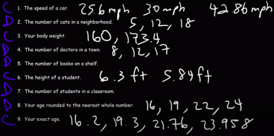
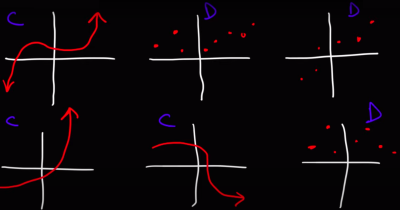


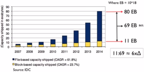
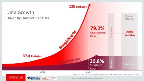


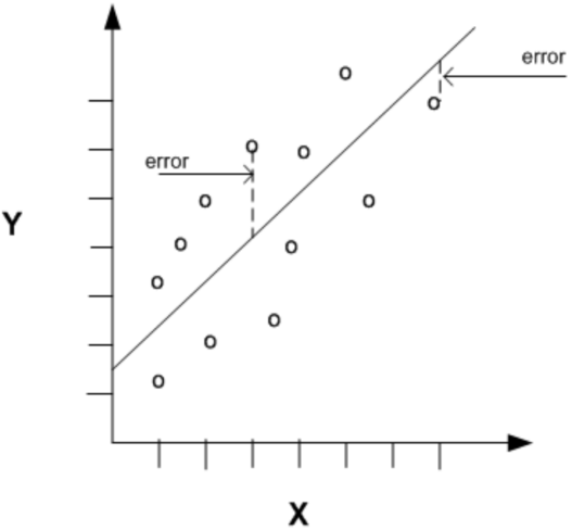


